Understanding BI Server Runtime Performance

The BI Server is a runtime service that can be asked to maintain large amounts of data in memory. As a user, you can take steps to boost BI Server performance and to maintain consistent levels of runtime performance. Having an understanding of its internals will greatly help you optimize runtime operations.

The BI Server is a lightweight, read-optimized, in-memory only database. This means that data ingested in online data models is entirely loaded inside the BI Server process and queries are executed against the BI Server memory storage. To keep memory consumption at the minimal possible levels, the BI Server is designed to be a columnar database: table data is not stored in a row layout, but instead columns are stored individually. Since columns are essentially long lists of values of the same data type, they can be easily and efficiently compressed using lightweight compression schemes. The columnar layout also allows for increased efficiency in query execution, as columns can be scanned individually without having to process the entire row.

Memory Usage

The BI Server employs several compression techniques to reduce the memory footprint of a column, but as a rule of thumb the lower the column cardinality (number of unique values) the better the compression will be. When creating data flows for ingesting data into models, consider dropping any column that will not be used in runtime, especially high cardinality columns (such as identifiers). For numeric columns, consider dropping non-significant decimal digits by configuring the data flow to round the value using a Transform Column step and the roundto function, as this might reduce the column’s cardinality.

Sorted columns offer even more opportunities for compression, as they usually contain long runs of the same value and lend themselves well to be compressed using Run-Length Encoding. Run-Length Encoding represents a run of a value with just a triple: the value itself, the number of repetitions and the position of the first occurrence, which saves memory the longer the runs are.

For example, let’s assume that we have imported one year’s worth of historical data logged at 15 minutes interval for 1,000 tags. This translates to a table with just a little over 35 million rows. If all the values have good quality, the Quality column in the table will contain 35 million zeros. This can be stored using Run-Length Encoding with just three integers [0; 35,040,000; 0]—a compression ratio of over 99%. For this reason, consider pre-sorting data on applicable attributes before ingesting it into a data model.

Query Execution and Cache

When writing a query is it recommended to only select the necessary attributes as needed in the resulting dataset, as this will improve the query execution.

The BI Server employs a temporary cache for query results. Results of a query are stored in the cache using the query itself as a key. This means that if two different clients request the same query, then that query will only be executed once. After the first execution, the result is cached, and subsequent requests will receive the result from the cache. This is especially important when subscribing to BI Server queries as individual data element requests rather than entire datasets.

For example, let’s assume that we want to display the average product unit price per category with in several process points in GraphWorX. We could use the following set of point names to get these results, specifying the CategoryID in each query:

• bi:Models:Northwind(SELECT AVG(Products.UnitPrice), Products.CategoryID WHERE Products.CategoryID = 1)[UnitPrice][0]
• bi:Models:Northwind(SELECT Categories.CategoryName WHERE Categories.CategoryID = 1)[CategoryName][0]
• bi:Models:Northwind(SELECT AVG(Products.UnitPrice), Products.CategoryID WHERE Products.CategoryID = 2)[UnitPrice][0]
• bi:Models:Northwind(SELECT Categories.CategoryName WHERE Categories.CategoryID = 2)[CategoryName][0]

. . .

• bi:Models:Northwind(SELECT AVG(Products.UnitPrice), Products.CategoryID WHERE Products.CategoryID = 8)[UnitPrice][0]
• bi:Models:Northwind(SELECT Categories.CategoryName WHERE Categories.CategoryID = 8)[CategoryName][0]

The result is that we are submitting 16 different queries to the BI Server to get the value for our process points. Each query returns a single column and single row. This is not necessarily an issue; however, we can improve performance by taking advantage of the BI Server cache. The results shown above can all be produced in a single dataset by the following query:

This will return all of the data we want in a single dataset of two columns and eight rows. We can then display individual elements in from dataset with our process points in the following way:

• bi:Models:Northwind(SELECT AVG(Products.UnitPrice), Categories.CategoryName, Categories.CategoryID ORDER BY Categories.CategoryID)[UnitPrice][0]
• bi:Models:Northwind(SELECT AVG(Products.UnitPrice), Categories.CategoryName, Categories.CategoryID ORDER BY Categories.CategoryID)[CategoryName][0]

. . .

• bi:Models:Northwind(SELECT AVG(Products.UnitPrice), Categories.CategoryName, Categories.CategoryID ORDER BY Categories.CategoryID)[UnitPrice][7]
• bi:Models:Northwind(SELECT AVG(Products.UnitPrice), Categories.CategoryName, Categories.CategoryID ORDER BY Categories.CategoryID)[CategoryName][7]

Now all 16 points are executing the exact same query, and each point is specifying a different row or column from the query results. This means that BI Server will only have to execute the query once, cache it, and then serve the cached results to all sixteen process points.

Miscellaneous Performance Boosting Tips

• Optimize your Data Flows by following a few simple steps:

  1. Only import the columns from the data source that you are actually planning to use. Delete all not referenced columns.
  2. When importing historical data try to reduce the volume of historical data by importing aggregations of the raw historical data when possible (for example daily data over a month period).

• Optimize your Data Tables by following a few simple steps:

  1. Always define a Primary Key in your data table to safeguard data integrity.
  2. Define relationships between your data tables to enable the BI Server to process queries much more efficiently if those queries would otherwise require JOIN functions.
  3. Always control the size of a data table by safeguarding the number of records using triggers to control data refreshes and incremental updates. Make sure that no data table is set to increase in number of records indefinitely.

• Customize your Data Load time for volume of data and types of data sources

  1. By default, BI Server uses a default Data Load timeout of 120 seconds. Although this is sufficient for a number of cases, it may be necessary to adjust it.
  2. You can adjust the Data Load timeout setting, by using the Platform Services Configuration form inside Workbench.

BI Server Runtime Parameters

There are some important BI Server runtime parameters that impact the data loading operations and overall performance. In this section, we will analyze a few important parameters that are related exclusively to the data load operations. To view or edit the above parameters, you will need to navigate to the Workbench Ribbon and click on the Platform Services Configuration under Tools.

When you click on the Platform Services Configuration button, the related form will be displayed. You will need to select the BI Server Point Manager from the list of Point Managers.

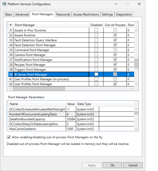
The data load-related parameters can be found under the Point Manager Parameters section. The important parameters relating to data loading are:

• NumberOfConcurrentLoadingTasks: Each Data Table in an online Data model triggers a loading task to ingest the table’s data when the server starts up. This parameter defines how many loading tasks the BI Server can run concurrently. The default is 4.

• DataLoadTimeoutSec: Defines the time, in seconds, after which a loading task will be considered timed out and then aborted. Loading tasks process the data in chunks of rows (see DataflowBoundedCapacity parameter) and this timeout value applies to reading a single chunk of data from the Data Flow, after which it will reset to read the next chunk. Please note that there is a notable exception for Data Flows using the Transpose Step, as this step must consume the entire input before producing its output which means that this parameter value must be made large enough for the Transpose Step to have the time to consume the entire input data source. A loading task that times out is not retried. The retry count and retry delay below do not apply to loading tasks that have timed out. The default value is 120.

• DataLoadRetryCount: Defines how many times to retry a loading task if the task fails (returns an error or has an exception). The default value is 3.

• DataLoadRetyDelayMsec: Defines the amount of time to wait, in milliseconds, after a loading task failure before retrying. The default value is 10000.

• DataflowBoundedCapacity: Defines how many rows are requested at the time from the data source associated with the Data Table. The default value is 16384.